利用加速度求解位置的算法——三轴传感器

摘要

    此文档描述并使用MMA7260QT三轴加速计和低功耗的9S08QG8八位单片机实现求解位置的算法 。

    在今天先进的电子市场，有不少增加了许多特性和智能的多功能的产品。定位和游戏只是得益于获取到的位置信息的一部分市场。一个获取这种信息的可选方案是通过使用惯性传感器。从这些传感器中取得的信号需要进行一些处理，因为在加速度和位置之间没有一种直接转换。

    为了获得位置，需要对加速度进行二次积分。本文介绍一种简单的算法实现加速度的二重积分。为了获取加速度的二重积分，一个简单的积分要进行两次，因为这样也可以顺便获取速度。

    接下来要展示的算法，能够应该于任何传感轴，所以一维、二维、三维的位置都可以被计算出。当在获取三维位置信息时，要特别地除去重力加速度的影响。下面的算法实现还包括了一个二维系统的例子（比如鼠标）。

应用潜力

    这种算法的应用潜力在于个人导航、汽车导航和（back-up）GPS、防盗设备、地图追踪、3D游戏、计算机鼠标等等。这类产品都需要用到求解位置信息的算法。

    本文所介绍的算法在位移精度要求不是很严格的情况下很有用。其他的情况和影响特别是应用，当采用本文算法时，需要考虑一下。对最终程序进行微小的修改和调整，这种算法能够达到更高的精度。

理论知识和算法

     理解本文算法的最好方法是回顾一下数学上的积分知识。

    加速度是一个对象速度的变化速率。同时，速度是同样一个对象位置的变化速率。换句话说，速度是位置的导数，加速度是速度的导数，因此如下公式：

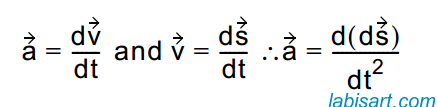
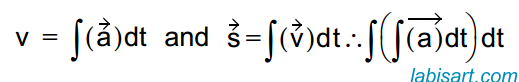
    积分和导数相反。如果一个物体的加速度已知，那么我们能够利用二重积分获得物体的位置。假设初始条件为0，那么有如下公式：

    一个理解这个公式的方法是将积分定义成曲线下面包围的区域，积分运算结果是极小区域的总和，区域的宽度趋近于0。换句话说，积分的和表示了一个物理变量的大小（速度）。

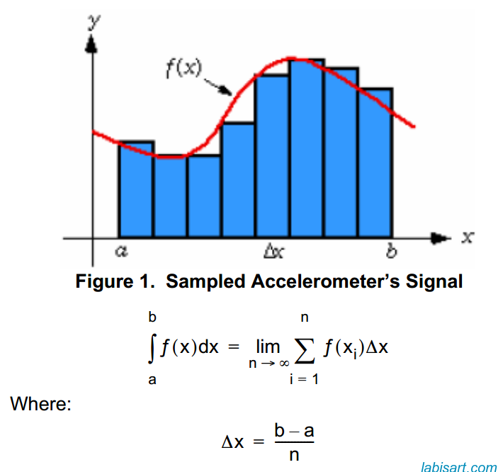
    利用前面的一个概念——曲线下面的区域，我们能得出一个结论：对一个信号采样，得到该信号大小的瞬时值，所以能够在两次采样之间得到一个小的区域。为了获得连贯的值采样时间必须相同。采样时间代表这块区域的宽，同时采样得到的值代表区域的高。为了消除带有分数的乘法（微秒或毫秒），我们假定时间为一个单位。

    现在，我们知道了每个代表区域宽度的采样时间等于1。下一个结论是：

    积分的值可以约等于区域面积之和。

    如果采样时间趋近于0，那么结论将是正确的。但在实际中，将会产生如下错误，在处理的过程中，这个误差将会一直累积。

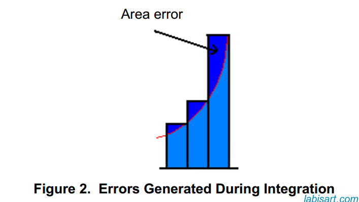
      这些错误称为采样损失。为了减少这些错误，我们再做进一步的假设。结果区域能够看成由两块小的区域的组合：

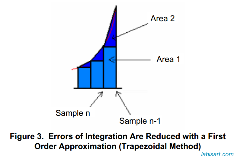
    区域1是前一次采样的值（方形），区域2是一个三角形，是前一次采样和当前采样之差的一半。

    通过这种方法，我们现在有一个一阶近似（插值）的信号。

    现在的错误比以前的近似的低得多。

    尽管加速度有正有负，但采样的值总是正的（基于MMA7260QT的输出特性），因此需要做一个偏移判断，换句话说，需要一个参考。这个程序即为校准程序。

    校准程序用于在没有移动情况下的加速度值上。这时，获得的加速度值可以看成是零参考点。低于零参考点的值代表负值（减速），高于零参考点的值代表正值（加速）。

    加速度计的输出范围为0v到Vdd，并且它通常由AD转换器得到。0值接近Vdd/2。前面获得的校准值会被芯片的方向和分解在各轴的静态加速度（重力加速度）所影响。如果装置刚好平行于地球表面，那么校准值将会很接近Vdd/2。

    接下来的这张图用于展示校准程序的结果。

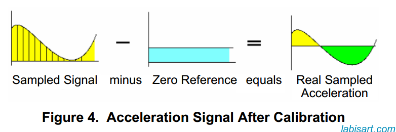
    从采样的信号减去零参考值，我们获得真正的采样加速度。

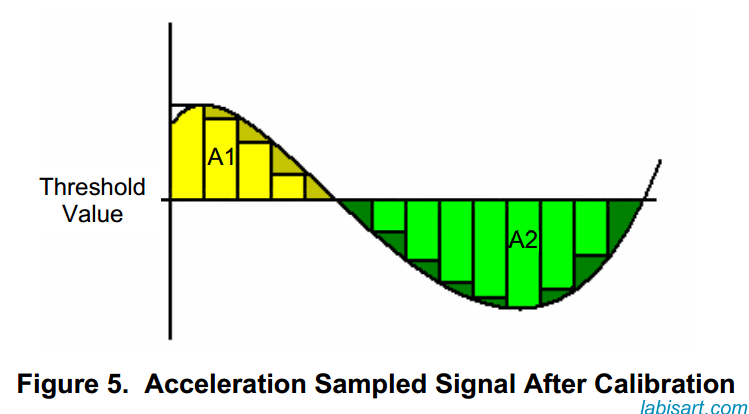
    A1代表正加速度，A2代表负加速度。

    如果我们将这数据看作是采样数据，那么信号值将和下图非常接近。

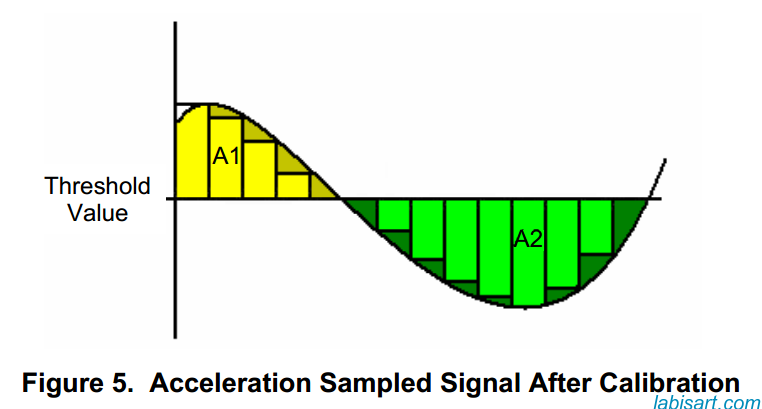
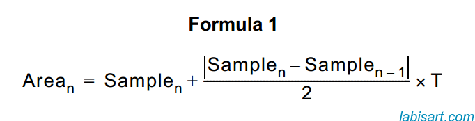
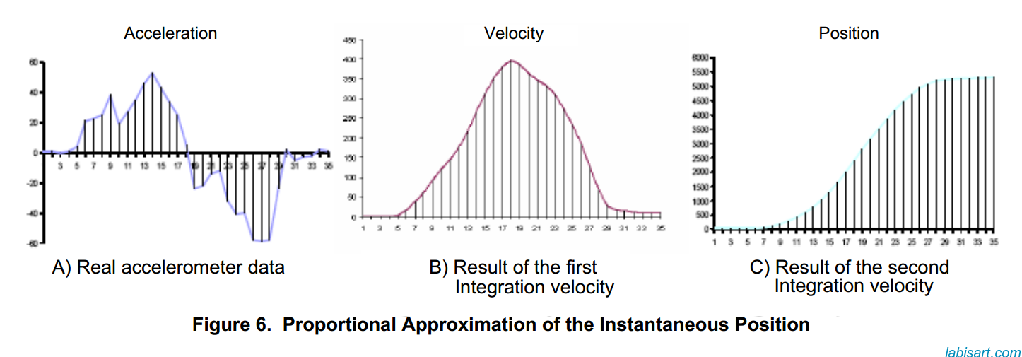
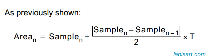
    通过使用上面的积分公式，Formula 1，我们将获得速度的比例近似值。同样，为了获取位置，需要再进行一次积分。在获得的速度数值上应用相同的公式和步骤，我们现在获得了一个瞬时位置的比例近似值。（见图6）

软件设计相关注意事项

    当在现实世界的实现中应用这种算法，应该考虑一下下面的步骤和建议。

•     信号存在一定的噪声，所以信号必须经过数字滤波。本算法中的滤波是一种移动平均算法，要处理的值是一定数量采样值的平均结果。

•     即使以前过滤的一些数据可能由于机械噪声导致错误，所以必须实现另一个滤波器。根据过滤的样品数，一个真实加速度的窗口能够被选择（一般为16±2采样次数）。

•     无运动状态对获得正确的数据是至关重要的。校准例程需要在应用程序的开头。该校准值必须尽可能准确。

•     加速度的真实值等于采样值减去校准值；它可以是正数或负数。当你在定义变量的时候，这绝对不能被忽略，需要定义为有符号数。

•     更快的采样频率意味着更精确的结果，因为采样频率越快误差越少。但是需要更多的内存、时间和硬件方面的考虑。

•     两次采样之间的时间必须要相同。如果这个时间不相同，将会产生错误。

•     两次采样结果之间的线性近似值（插值）被推荐用于更精确的结果。

代码注释

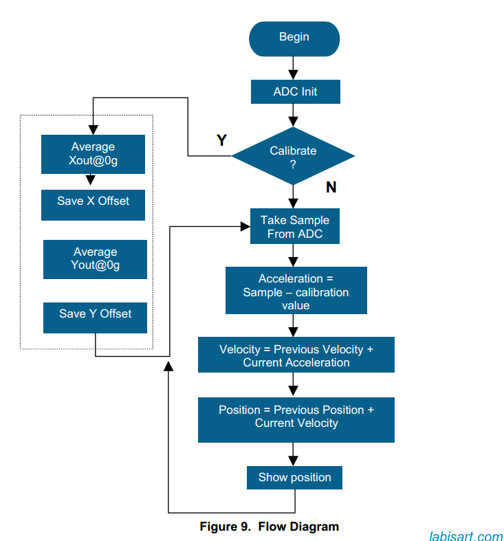
1. 校准程序

    这个校准程序移除了加速度传感器的输出偏移分量，因为存在重力加速度（静态的加速度）。

    校准程序在加速度计处于无运动状态时，对加速度求平均值。采样的数量越多，加速度的校准结果越精确。

voidCalibrate(void)
{
    unsignedint count1;
    count1 =0;
    do{
    ADC_GetAllAxis();
    sstatex = sstatex +Sample_X;// Accumulate Samples
    sstatey = sstatey +Sample_Y;
    count1++;
    }while(count1!=0x0400);// 1024 times
    sstatex=sstatex>>10;// division between 1024
    sstatey=sstatey>>10;
}

2. 滤波

    低通滤波是消除加速度计中信号噪音(包括机械的和电子的)很好的方法。为了当对信号进行积分时减少大部分的错误，减少噪音对定位应用是至关重要的。

    一个简单的低通过滤采样信号的方式是执行滚动平均值。过滤简单地获得一组采样的平均值，获得稳定的采样总数的平均值是很重要的。采样数太多可能造成数据丢失，而太少又可能导致结果不精确。

do{
    accelerationx[1]=accelerationx[1]+Sample_X;//filtering routine for noise attenuation
    accelerationy[1]=accelerationy[1]+Sample_Y;//64 samples are averaged. The resulting
    count2++;// average represents the acceleration of
    // an instant.
}while(count2!=0x40);// 64 sums of the acceleration sample
accelerationx[1]= accelerationx[1]>>6;// division by 64
accelerationy[1]= accelerationy[1]>>6;

3. 机械滤波窗口

    当处于无运动状态时，加速度上的微小错误可能会被当作一个常量速度，因为在采样值加和之后，它并不等于0。在没有运动的理想情况下，所有的采样值都为0。该常速表示一个连续的移动和不稳定的位置。

    即使之前过滤的一些数据可能不正确，因此一个用于区别无运动状态的"有效数据"和"无效数据"的窗口必须实现。

if ((accelerationx[1] <=3)&&(accelerationx[1] >= -3)) //Discrimination window applied to
{
    accelerationx[1] = 0;
} // the X axis acceleration variable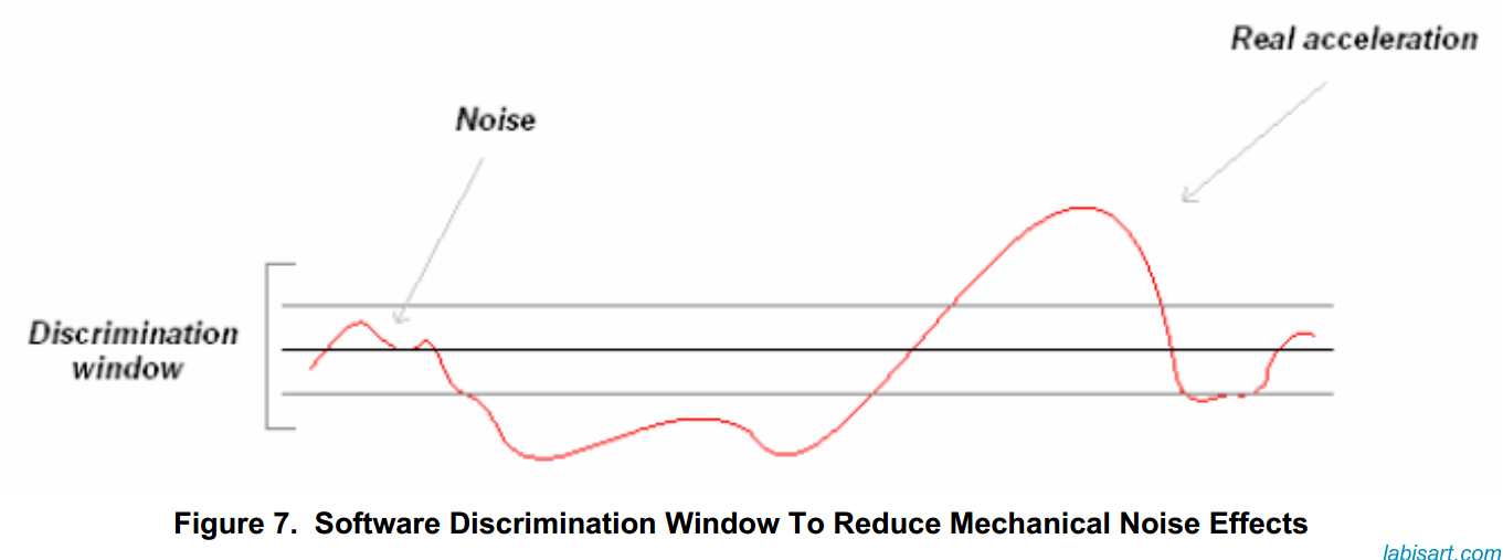

4. 定位

    二重积分是利用加速度数据获取位置所需要的步骤。第一次积分获得速度，第二次积分获得位置。

//first integration
 velocityx[1]= velocityx[0]+ accelerationx[0]+((accelerationx[1]- accelerationx[0])>>1)
//second integration
 positionX[1]= positionX[0]+ velocityx[0]+((velocityx[1]- velocityx[0])>>1);

5. 数据传输

    这部分主要目的是用于调试和显示；这个函数中32位的结果被切割分4个8位数据。

if (positionX[1]>=0) 
{ //This line compares the sign of the X direction data
    direction= (direction | 0x10); // if its positive the most significant byte
    posx_seg[0]= positionX[1] & 0x000000FF; // is set to 1 else it is set to 8
    posx_seg[1]= (positionX[1]>>8) & 0x000000FF; // the data is also managed in the
    // subsequent lines in order to be sent.
    posx_seg[2]= (positionX[1]>>16) & 0x000000FF;// The 32 bit variable must be split into
    posx_seg[3]= (positionX[1]>>24) & 0x000000FF;// 4 different 8 bit variables in order to
    // be sent via the 8 bit SCI frame
}
else 
{
    direction=(direction | 0x80);
    positionXbkp=positionX[1]-1;
    positionXbkp=positionXbkp^0xFFFFFFFF;
    posx_seg[0]= positionXbkp & 0x000000FF;
    posx_seg[1]= (positionXbkp>>8) & 0x000000FF;
    posx_seg[2]= (positionXbkp>>16) & 0x000000FF;
    posx_seg[3]= (positionXbkp>>24) & 0x000000FF;
}

6. "移动结束"检查

    基于积分表示曲线下方区域的概念，速度是加速曲线下方的区域的结果。

    如果我们观察一个典型的移动:一个物体沿一个轴从点A移动到点B，一个典型的加速度结果如下图:

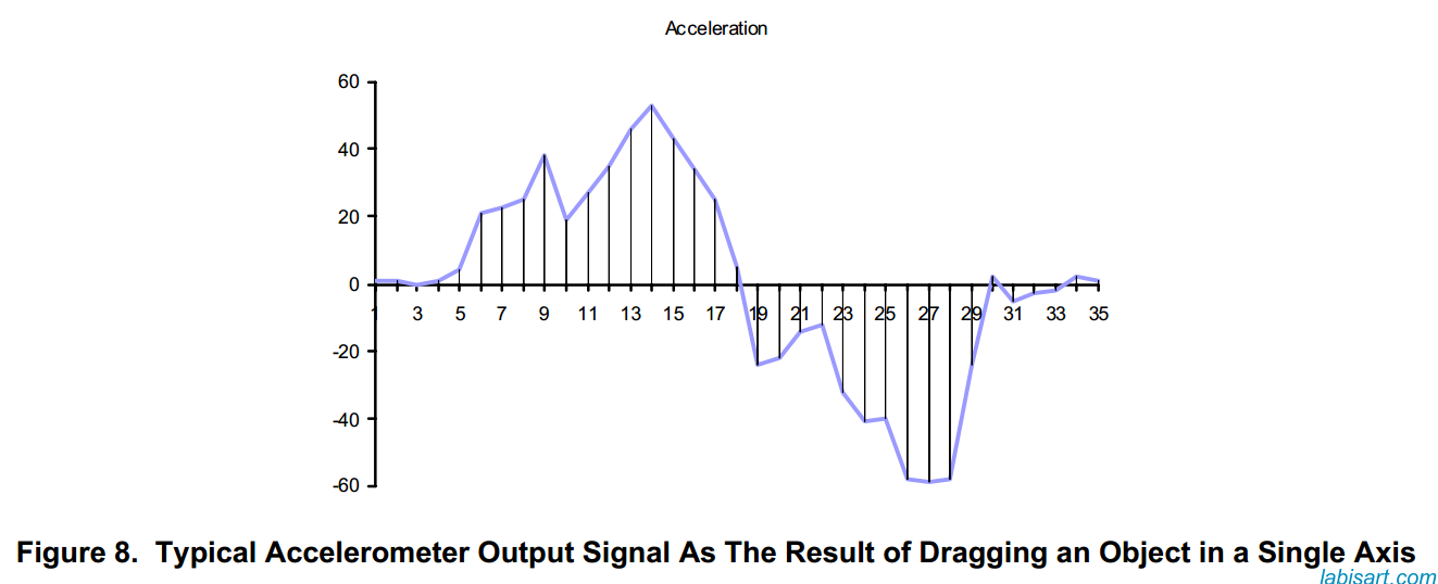
    观察上面的图，加速度先增加后减少直到速度达到最大值（加速度始终为正代表往同一方向加速）。然后以相反的方式加速，直到它再次到达0。在这一点上达到一个稳定的位移和新的位置。

    在真实世界中，其中曲线正侧下方的区域面积不等于负侧上方的区域面积，积分结果将永远不会达到零速度，因此将是一个倾斜定位（从未稳定）。

    正因为如此，将速度强制减为0非常关键。这是通过不断读取加速度值和0进行比较而实现的。如果在一定数量的采样中，这种情况存在（sample==0）的话，速度将简单地返回为0。

if (accelerationx[1]==0) // we count the number of acceleration samples that equals zero
{ 
    countx++;
}
else 
{ 
    countx =0;
}
if (countx>=25) // if this number exceeds 25, we can assume that velocity is zero
{
    velocityx[1]=0;
    velocityx[0]=0;
}

7. 源代码

#include <hidef.h>
#include "derivative.h"
#include "adc.h"
#include "buzzer.h"
#include "SCItx.h"
#pragma DATA_SEG MY_ZEROPAGE
unsigned char near Sample_X;
unsigned char near Sample_Y;
unsigned char near Sample_Z;
unsigned char near Sensor_Data[8];
unsigned char near countx,county ;
signed int near accelerationx[2], accelerationy[2];
signed long near velocityx[2], velocityy[2];
signed long near positionX[2];
signed long near positionY[2];
signed long near positionZ[2];
unsigned char near direction;
unsigned long near sstatex,sstatey;
#pragma DATA_SEG DEFAULT
void init(void);
void Calibrate(void);
void data_transfer(void);
void concatenate_data(void);
void movement_end_check(void);
void position(void);
void main (void)
{
 init();
 get_threshold();
 do
 {
 position();
 }while(1);
}
/*******************************************************************************
 The purpose of the calibration routine is to obtain the value of the reference threshold.
 It consists on a 1024 samples average in no-movement condition.
********************************************************************************/
void Calibrate(void)
{
 unsigned int count1;
 count1 = 0;
 do{
 ADC_GetAllAxis();
 sstatex = sstatex + Sample_X; // Accumulate Samples
 sstatey = sstatey + Sample_Y;
 count1++;
 }while(count1!=0x0400); // 1024 times
 sstatex=sstatex>>10; // division between 1024
 sstatey=sstatey>>10;
}
/*****************************************************************************************/
/******************************************************************************************
This function obtains magnitude and direction
In this particular protocol direction and magnitude are sent in separate variables.
Management can be done in many other different ways.
*****************************************************************************************/
void data_transfer(void)
{
 signed long positionXbkp;
 signed long positionYbkp;
 unsigned int delay;
 unsigned char posx_seg[4], posy_seg[4];
 if (positionX[1]>=0) { //This line compares the sign of the X direction data
 direction= (direction | 0x10); //if its positive the most significant byte
 posx_seg[0]= positionX[1] & 0x000000FF; // is set to 1 else it is set to 8
 posx_seg[1]= (positionX[1]>>8) & 0x000000FF; // the data is also managed in the
 // subsequent lines in order to
 posx_seg[2]= (positionX[1]>>16) & 0x000000FF; // be sent. The 32 bit variable must be
 posx_seg[3]= (positionX[1]>>24) & 0x000000FF; // split into 4 different 8 bit
 // variables in order to be sent via
 // the 8 bit SCI frame
}
 else {direction=(direction | 0x80);
 positionXbkp=positionX[1]-1;
 positionXbkp=positionXbkp^0xFFFFFFFF;
 posx_seg[0]= positionXbkp & 0x000000FF;
 posx_seg[1]= (positionXbkp>>8) & 0x000000FF;
 posx_seg[2]= (positionXbkp>>16) & 0x000000FF;
 posx_seg[3]= (positionXbkp>>24) & 0x000000FF;
 }
 if (positionY[1]>=0) { // Same management than in the previous case
 direction= (direction | 0x08); // but with the Y data.
 posy_seg[0]= positionY[1] & 0x000000FF;
 posy_seg[1]= (positionY[1]>>8) & 0x000000FF;
 posy_seg[2]= (positionY[1]>>16) & 0x000000FF;
 posy_seg[3]= (positionY[1]>>24) & 0x000000FF;
 }
 else {direction= (direction | 0x01);
 positionYbkp=positionY[1]-1;
 positionYbkp=positionYbkp^0xFFFFFFFF;
 posy_seg[0]= positionYbkp & 0x000000FF;
 posy_seg[1]= (positionYbkp>>8) & 0x000000FF;
 posy_seg[2]= (positionYbkp>>16) & 0x000000FF;
 posy_seg[3]= (positionYbkp>>24) & 0x000000FF;
 }
 delay = 0x0100;
 Sensor_Data[0] = 0x03;
 Sensor_Data[1] = direction;
 Sensor_Data[2] = posx_seg[3];
 Sensor_Data[3] = posy_seg[3];
 Sensor_Data[4] = 0x01;
 Sensor_Data[5] = 0x01;
 Sensor_Data[6] = END_OF_FRAME;
 while (--delay);
 SCITxMsg(Sensor_Data); // Data transferring function
 while (SCIC2 & 0x08);
}
/*****************************************************************************************/
/******************************************************************************************
This function returns data format to its original state. When obtaining the magnitude and
direction of the position, an inverse two's complement is made. This function makes the two's
complement in order to return the data to it original state.
It is important to notice that the sensibility adjustment is greatly impacted here, the amount
of "ones" inserted in the mask must be equivalent to the "ones" lost in the shifting made in
the previous function upon the sensibility modification.
 ******************************************************************************************/
void data_reintegration(void)
{
 if (direction >=10)
{positionX[1]= positionX[1]|0xFFFFC000;} // 18 "ones" inserted. Same size as the
 //amount of shifts
 direction = direction & 0x01;
 if (direction ==1)
 {positionY[1]= positionY[1]|0xFFFFC000;}
}
/******************************************************************************************
This function allows movement end detection. If a certain number of acceleration samples are
equal to zero we can assume movement has stopped. Accumulated Error generated in the velocity
calculations is eliminated by resetting the velocity variables. This stops position increment
and greatly eliminates position error.
******************************************************************************************/
void movement_end_check(void)
{
 if (accelerationx[1]==0) //we count the number of acceleration samples that equals cero
 { countx++;}
 else { countx =0;}
 if (countx>=25) //if this number exceeds 25, we can assume that velocity is cero
 {
 velocityx[1]=0;
 velocityx[0]=0;
 }
 if (accelerationy[1]==0) //we do the same for the Y axis
 { county++;}
 else { county =0;}
 if (county>=25)
 {
 velocityy[1]=0;
 velocityy[0]=0;
 }
}
/*****************************************************************************************/
/******************************************************************************************
This function transforms acceleration to a proportional position by integrating the
acceleration data twice. It also adjusts sensibility by multiplying the "positionX" and
"positionY" variables.
This integration algorithm carries error, which is compensated in the "movenemt_end_check"
subroutine. Faster sampling frequency implies less error but requires more memory. Keep in
mind that the same process is applied to the X and Y axis.
*****************************************************************************************/
void position(void)
{
unsigned char count2 ;
count2=0;
 do{
 ADC_GetAllAxis();
 accelerationx[1]=accelerationx[1] + Sample_X; //filtering routine for noise attenuation
 accelerationy[1]=accelerationy[1] + Sample_Y; //64 samples are averaged. The resulting
//average represents the acceleration of
 //an instant
 count2++;
 }while (count2!=0x40); // 64 sums of the acceleration sample
 accelerationx[1]= accelerationx[1]>>6; // division by 64
 accelerationy[1]= accelerationy[1]>>6;
 accelerationx[1] = accelerationx[1] - (int)sstatex; //eliminating zero reference
 //offset of the acceleration data
 accelerationy[1] = accelerationy[1] - (int)sstatey; // to obtain positive and negative
 //acceleration
 if ((accelerationx[1] <=3)&&(accelerationx[1] >= -3)) //Discrimination window applied
 {accelerationx[1] = 0;} // to the X axis acceleration
 //variable
 if ((accelerationy[1] <=3)&&(accelerationy[1] >= -3))
 {accelerationy[1] = 0;}
 //first X integration:
velocityx[1]= velocityx[0]+ accelerationx[0]+ ((accelerationx[1] -accelerationx[0])>>1);
 //second X integration:
positionX[1]= positionX[0] + velocityx[0] + ((velocityx[1] - velocityx[0])>>1);
 //first Y integration:
velocityy[1] = velocityy[0] + accelerationy[0] + ((accelerationy[1] -accelerationy[0])>>1);
 //second Y integration:
positionY[1] = positionY[0] + velocityy[0] + ((velocityy[1] - velocityy[0])>>1);
 accelerationx[0] = accelerationx[1]; //The current acceleration value must be sent
//to the previous acceleration
 accelerationy[0] = accelerationy[1]; //variable in order to introduce the new
//acceleration value.
 velocityx[0] = velocityx[1]; //Same done for the velocity variable
 velocityy[0] = velocityy[1];
 positionX[1] = positionX[1]<<18; //The idea behind this shifting (multiplication)
 //is a sensibility adjustment.
 positionY[1] = positionY[1]<<18; //Some applications require adjustments to a
 //particular situation
 //i.e. mouse application
 data_transfer();
 positionX[1] = positionX[1]>>18; //once the variables are sent them must return to
 positionY[1] = positionY[1]>>18; //their original state
 movement_end_check();
 positionX[0] = positionX[1]; //actual position data must be sent to the
 positionY[0] = positionY[1]; //previous position
 direction = 0; // data variable to direction variable reset
}
/*****************************************************************************************/

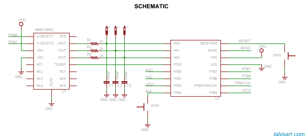
原理图

总结

    本文档为利用加速度计实现定位算法提供了一些基本的概念。

    这种特定的算法在对位移精度要求不是很严格中非常有用。其他注意事项和具体的应用程序的影响应该在实现这个示例时被考虑。

    这种积分算法适合于低端嵌入式应用，因为它的简单性和少量的指令。它也没有涉及任何浮点运算。

原文链接：http://cache.freescale.com/files/sensors/doc/app_note/AN3397.pdf
转载链接：http://www.cnblogs.com/cposture/p/4378922.html

• 上一篇： MFC非模态对话框无焦点对话框使用PreTranslateMessage做加速键
• 下一篇： STM32F30x 固件库下载地址 F303